ABSTRACT
We describe a new approach to multiple sequence alignment using
genetic algorithms and an associated software package called SAGA. The
method involves evolving a population of alignments in a quasi evolutionary
manner and gradually improving the fitness of the population as measured
by an objective function which measures multiple alignment quality. SAGA
uses an automatic scheduling scheme to control the usage of 22 different
operators for combining alignments or mutating them between generations.
When used to optimise the well known sums of pairs objective function,
SAGA performs better than some of the widely used alternative packages.
This is seen with respect to the ability to achieve an optimal solution
and with regard to the accuracy of alignment by comparison with reference
alignments based on sequences of known tertiary structure. The general
attraction of the approach is the ability to optimise any objective function
that one can invent.
The simultaneous alignment of many nucleic acid or amino acid sequences is one of the most commonly used techniques in sequence analysis. Multiple alignments are used to help predict the secondary or tertiary structure of new sequences; to help demonstrate homology between new sequences and existing families; to help find diagnostic patterns for families; to suggest primers for PCR and as an essential prelude to phylogenetic reconstruction. The great majority of automatic multiple alignments are now carried out using the `progressive' of Feng and Doolittle ( 1 ) or variations on it ( 2 - 4 ). This approach has the great advantage of speed and simplicity combined with reasonable sensitivity as judged by the ability to align sets of sequences of known tertiary structure. The main disadvantage of this approach is the `local minimum' problem which stems from the greedy nature of the algorithm. This means that if any mistakes are made in any intermediate alignments, these cannot be corrected later as more sequences are added to the alignment. Further, there is no objective function (a measure of overall alignment quality) which can be used to say that one alignment is preferable to another or to say that the best possible alignment, given a set of parameters, has been found.
There are two main alternatives to progressive alignment. One is to use hidden Markov models (HMMs; 5 ) which attempt to simultaneously find an alignment and a probability model of substitutions, insertions and deletions which is most self consistent. Currently, this approach is limited, in practice, to cases with very many sequences (e.g. 100 or more) but does have the great advantage of a sound link with probability analysis. A second approach is to use objective functions (OFs) which measure multiple alignment quality and to find the best scoring alignment. If the OF is well chosen or is an accurate measure of quality, then this approach has the advantage that one can be confident that the resulting alignment really is the best by some criterion. Unfortunately, the number of possible alignments which must be scored in order to choose the best one becomes astronomical for more than four or five sequences of reasonable length.
Two solutions to this problem exist. The MSA program ( 6 , 7 ) attempts to narrow down the solution space to a relatively small area where the best alignment is likely to be. It then guarantees finding the best alignment in this reduced space. Even with this reduction, it is limited to small examples of around seven or eight sequences at most. Nonetheless, it is the only method we know of that seems capable of finding the globally optimal alignment or close to it, starting with completely unaligned sequences. A second approach is to use stochastic optimisation methods such as simulated annealing ( 8 ), Gibbs sampling ( 9 ) or genetic algorithms (GAs; 10 ). Simulated annealing has been used on numerous occasions for multiple alignment (e.g. 11 - 13 ) but can be very slow and usually only works well as an alignment improver i.e. when the method is given an alignment that is already close to optimal and is not trapped in a local minimum. Gibbs sampling has been very successfully applied to the problem of finding the best local multiple alignment block with no gaps but its application to gapped multiple alignment is not trivial. Finally, we know of one attempt at using GAs in this context ( 14 ). Here they used a hybrid iterative dynamic programming/GA scheme.
In this paper, we describe a GA strategy and software package called
SAGA (sequence alignment by genetic algorithm) which appears capable of
finding globally optimal multiple alignments (or close to it) in reasonable
time, starting from completely unaligned sequences. It can find solutions
that are as good as or better than either MSA or CLUSTAL W ( 3
) as measured by the OF score or by reference to alignments of sequences
of known tertiary structure. The approach has a further advantage in that
it can be used to optimise any OF one can invent. Biologically, the key
to successful application of optimisation methods to this problem, depends
critically on the OF. If the OF is not a good descriptor of multiple alignment
quality, then the alignments will not necessarily be best in any real sense.
The search for useful OFs for sequence alignment, perhaps for different
purposes, is surely a key area of research. Without SAGA, however, it is
difficult to consider most new OFs as one cannot optimise them.
The overall approach is to use a measure of multiple alignment quality
(an OF) and to optimise it using a genetic algorithm. A set of well known
test cases is used as a reference to evaluate the efficiency of the optimisation.
Evaluation of the alignments is made using an OF which is simply a measure of multiple alignment quality. We use two OFs related to the weighted sums of pairs with affine gap penalties ( 15 ). The principle is to give a cost to each pair of aligned residues in each column of the alignment (substitution cost), and another cost to the gaps (gap cost). These are added to give the global cost of the alignment. Furthermore, each pair of sequences is given a weight related to their similarity to the other pairs. Variations involve: (i) using different sets of sequence weights; (ii) different sets of costs for the substitutions [e.g. PAM matrices ( 16 ) or BLOSUM tables ( 17 )]; (iii) different schemes for the scoring of gaps ( 18 ). The cost of a multiple alignment (A) is then: A L I G N M E N T ^ C O S T ( A ) = {sum from {i = 2} to N} {sum from {j = 1} to {i - l}} {W sub {i , j}} " " C O S T {{( A} sub i} , {A sub j} )
where COST is the alignment score between two aligned sequences (A i and A j ) and W i,j is their weight. The COST function includes gap opening and extension penalties for opening and extending gaps. Altschul ( 18 ) made an extensive review describing the different ways of scoring gaps in a multiple alignment. Two different methods were used in SAGA: (i) natural affine gap penalties and (ii) quasi-natural affine gap penalties. These methods differ in how they treat nested gaps, i.e. a gap in one sequence that is completely contained in the second. In both cases, positions where both sequences have a null are removed. With the natural gap penalties, gap opening and extension penalties are charged for each remaining gap. With the quasi-natural gap penalties, an additional gap opening penalty is charged for any gap in one sequence that starts after and ends before a gap in the second sequence (before the columns of null are removed). Terminal gaps are penalised for extension but not for opening.
Sequence weights are an attempt to minimise redundant information, based on the relatedness of the sequences. In MSA, a weight for every pair of sequences is derived from a phylogenetic tree connecting the sequences. In CLUSTAL W ( 20 ), a weight is calculated for each sequence and the pair weight (W i,j ) for two sequences is simply their product. These weights differ in detail although both are designed for a similar purpose.
In this study we give results for the optimisation of two OFs: (i)
OF1 weighted sums of pairs using the pam250 weight matrix with quasi-natural
gap penalties and MSA, rationale 2, weights ( 19
). This is the function optimised by MSA. (ii) OF2 weighted sums of
pairs using the pam250 weight matrix with natural gap penalties and CLUSTAL
W weights ( 20
).
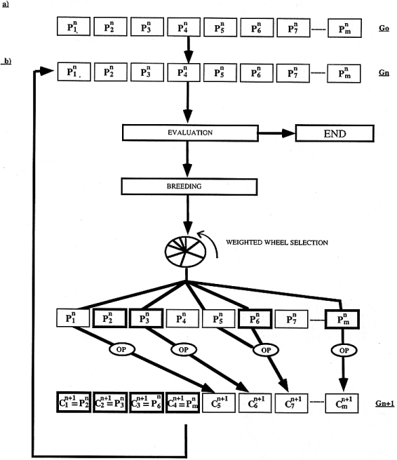
To align protein sequences, we designed a multiple sequence alignment method called SAGA. SAGA is derived from the simple genetic algorithm described by Goldberg ( 21 ). It involves using a population of solutions which evolve by means of natural selection. The overall structure of SAGA is shown in Figure 1 . The population we consider is made of alignments. Initially, a generation zero (G 0 ) is randomly created. The size of the population is kept constant. To go from one generation to the next, children are derived from parents that are chosen by some kind of natural selection, based on their fitness as measured by the OF (i.e. the better the parent, the more children it will have). To create a child, an operator is selected that can be a crossover (mixing the contents of the two parents) or a mutation (modifying a single parent). Each operator has a probability of being chosen that is dynamically optimised during the run.
Figure
These steps are repeated iteratively, generation after generation. During these cycles, new pieces of alignment appear because of the mutations and are combined by the crossovers. The selection makes sure that the good pieces survive and the dynamic setting of the operators helps the population to improve by creating the children it needs.
Following this simple process, the fitness of the population is increased until no more improvement can be made . All these steps, shown in Figure 1 , can be summarised by the following pseudo-code:
Initialisation 1. create G 0 Evaluation 2. evaluate the population of generation n (G n ) 3. if the population is stabilised then END 4. select the individuals to replace 5. evaluate the expected offspring (EO) Breeding 6. select the parent(s) from G n 7. select the operator 8. generate the new child 9. keep or discard the new child in G n+1 10. goto 6 until all the children have been success- fully put into G n+1 11. n = n+1 12. goto EVALUATION End 13. end Initialisation . The first step of the algorithm (Fig. 1 a) is the creation of a random population. This generation zero consists of a set of alignments containing only terminal gaps. A population size of 100 was used in all of the results presented here. To create one of these alignments, a random offset is chosen for all the sequences (the typical range being from 0 to 50 for sequences 200 residues long) and each sequence is moved to the right, according to its offset.The sequences are then padded with null signs in order to have the same length, L. The alignments of generation zero will be the parents of the children used to populate generation one. Evaluation. To give birth to a new generation, the first step is the evaluation of the fitness of each individual. This fitness is assessed by scoring each alignment according to the OF. The better the alignment, the better its score, and thus the higher its fitness. If the purpose is to minimise the OF, as is the case for OF1 and OF2, then the scores are inverted to give the fitness. The expected offspring (EO) of an alignment is derived from the fitness. It is typically a small integer. The method we used to derive it is known as remainder stochastic sampling without replacement ( 22 ). In the case of OF1 and OF2 the typical values of the EO are between 0 and 2, which can be considered as an acceptable range ( 21 ).
Only a portion (e.g. 50%) of the population is to be replaced during each generation. This technique, known as overlapping generation ( 23 ), means that half of the alignments will survive unchanged, the other half will be replaced by the children. We chose in SAGA to keep only the best individuals, and to replace the others. In practice, all the individuals are ranked according to their fitness, and the weakest are replaced by new children while creating the generation n+1 from the generation n. The other individuals (the fittest) will simply survive as they are during the breeding. Breeding. First, the new generation is directly filled with the fittest individuals from the previous generation (typically 50%). Next, the remaining 50% of the individuals in the new generation are created by selecting parents and modifying them. During the breeding, the EO is used as a probability for each individual to be chosen as a parent. A wheel is spun where each potential parent has a number of slots equal to its EO. When an individual is chosen to be a parent, its EO is accordingly decreased before the next turn of selection (selection without replacement). This weighted wheel selection is carried on until all the parents have been chosen.
To modify the parent(s), an operator has to be chosen. An operator is a small program that will modify an alignment (e.g. shuffle the gaps or merge two alignments into a new one). We have designed several operators. Each of them has a specific probability of being used. To create a child, one operator is chosen according to this probability (by spinning another weighted wheel). The chosen operator is then applied to the chosen parent(s). Some operators require two parents, others require only one.
An important aspect of the SAGA population structure is the constraint
we put on the absence of duplicates. In the same generation, all the alignments
have to be different. This technique helps maintain a high level of diversity
in a population of small size ( 24
). To do so, each newborn child is checked to ensure it is not identical
to any of the children already generated. If it is not, it will be put
into the new generation. Otherwise, it will simply be discarded along with
its parent(s) and the operator, in order to avoid deadlock problems. This
process is carried on until enough children (e.g. 50% of the population)
have been successfully inserted in the new generation. The Evaluation/Breeding
process will be carried on until the decision is made to stop the search.
End. There is no valid proof that a GA must reach the optimum,
even in an infinite amount of time, as there is for Simulated Annealing
( 25 ). Thus
the decision to stop the search has to be an arbitrary choice using more
or less sophisticated heuristic criteria. We use stabilisation as a criterion:
SAGA is stopped when the search has been unable to improve for some specified
number of generations (typically 100). This condition is the most widely
used when working on a population with no duplicates ( 26
).
According to the traditional nomenclature of genetic algorithms ( 21 ), two types of operators are represented in SAGA: the crossovers and the mutations. These programs perform modifications (mutation) or merging of parent alignments (crossover). In SAGA we do not make any distinction between these two types with regard to how we apply them. They are designed as independent programs that input one or two alignments (the parents) and output one alignment (the child). Each operator requires one or more parameters which specify where the operation is to be carried out. For example, an operator which inserts a new gap must be told where (at which position in the alignment) and in which sequences the gap is to be inserted.
The parameters of an operator may be chosen completely randomly in some range in which case the operator is said to be used in a stochastic manner. Alternatively, all except one of the parameters may be chosen randomly and the value of the remaining parameter will be fixed by exhaustive examination of all possible values. The value which yields the optimal fitness will be used. When an operator is applied in this way, it is said to be used in semi-hill climbing mode. Most of the SAGA operators may be used in either way. The crossovers. Crossovers are responsible for combining two different alignments into a new one. We implemented two different types of crossover: one-point and uniform. The one point crossover combines two parent alignments through a single exchange. Figure 2 outlines this mechanism. The first parent is cut straight at some randomly chosen position and the second one is tailored so that the right and the left pieces of each parent can be joined together while keeping the original sequence of amino acids. Any void space that appears at the junction point is filled with null signs. Because of the specificity of this junction point, where rearrangements can occur, this operator combines both the traditional properties of a crossover and those of a local rearrangement mutation. Only the best of the two children produced that way is kept.
Figure
This one point crossover can be very disruptive, especially at the junction point. To avoid this drawback, we added a second operator: the uniform crossover, designed to promote multiple exchanges between two parents in a more subtle manner. This operator is based on an analogy with biological crossover: exchanges are promoted between zones of homology.
The first step consists of mapping the alignment positions that are consistent between the two parents. In an alignment, a position is a column of residues or nulls stacked on top of each other. Two positions are said to be consistent between two alignments, if in each line they contain the same residue (by reference to the original sequence) or a null coming from the same gap (i.e. between the same residues). For instance, if in one line of a given position we have ALA125 and at the same line of a position in the other alignment we have ALA101 then the two position are not consistent. This process is outlined in Figure 3 . Blocks between consistent positions can be directly swapped. One can do so in a semi-hill climbing way, if only the best combination of blocks is chosen, or in a stochastic way, if the block to place between two consistent positions is randomly chosen between the two alignments. Both uniform crossovers, the semi-hill climbing one and the stochastic one, are implemented in SAGA.
Figure
Gap insertion. While the crossovers combine patterns, there is
still a need to generate these patterns. All the remaining operators were
designed to serve this purpose. The gap insertion operator is the simplest.
This operator extends alignments by inserting gaps. Its mechanism is detailed in Figure 4 . To keep the sequences aligned, each sequence will get a gap insertion of the same size. The sequences are split into two groups. Within each group, all the sequences get the insertion at the same position. The two groups are chosen, based on an underlying estimated phylogenetic tree between the sequences. The tree is randomly split into two sub-trees (Fig. 4 a). Each group consists of all the sequences in one of the two sub-trees. For one of the groups, a position is randomly chosen (Fig. 4 b). A gap of randomly chosen length is then inserted in each of the sequences of the group at the same position (P1 in Fig. 4 b). A gap of the same length is also inserted into all of the sequences of the second group at some position within a maximum distance from the first gap insertion (P2 in Fig. 4 b). This is the stochastic version of the block insertion operator.
Figure
The semi-hill climbing version of this operator is similar to the stochastic one described above but in this case, all the parameters except P1 (the position of the insertion in the first group of sequences) are chosen randomly and all possible values of P1 are tested. The value of P1 that gives the best scoring alignment is chosen.
In general, it is dangerous to assume that the topology of the underlying tree is correct. In the current usage, the main effect of an incorrect tree topology will be to slow the program down. The ability to find the globally optimal alignment should not be changed, just the speed at which the solution will be found. When two groups are chosen, using the tree, one of the groups can consist of a single sequence. This means that, eventually, all possible arrangements of gaps can be found, even if the tree topology is completely wrong. Ideally one would use fuzzy groupings based on the tree but which allows alternative groupings. Block shuffling. Generating an optimal arrangement after a gap insertion can often be a matter of shifting a gap to the left or to the right. Therefore we designed an operator that moves blocks of gaps or residues (but not both together) inside an alignment. Here, we depart from the usual definition of a block as a section of alignment containing no gaps, with all of the sub-sequences having the same length ( 27 ). For the purposes of this operator, we define a block of residues to be a set of overlapping stretches of residues from one or more sequences, each stretch being delimited by a gap or an end of a sequence. Each sub-sequence can be a different length but all sub-sequences must overlap. Similarly, a block of gaps is a set of overlapping gaps. An example of each is given in Figure 5 a. A block is chosen by first selecting one residue or gap position from the alignment and then deriving the block to which it belongs. These can be moved inside the alignment, to generate new configurations. Figure 5 b, c and d show some types of move that can be made inside an alignment. These moves are an extension of those proposed for a simulated annealing approach described by ( 12 ). The limits of this move are contained in the alignment itself. A gap can only be shifted until it merges with another gap. Similarly, a stretch of residues can only be shifted until it merges with another stretch of residues. We can enumerate the different ways these operations may be used as follows:
Figure
- Move a full block of gaps or a full block of residues. (Fig. 5 b). - Split the block horizontally and move one of the sub blocks to the left or to the right. The subdivision of a block is made according to the tree (cf. gap insertion operator) (Fig. 5 c). - Split the block vertically and move one half to the left or to the right (Fig. 5 d). - The move can be made in a semi-hill climbing way, looking for the best position, or in a stochastic manner.
These different combinations lead to a total of 16 possible operators, designed to shuffle gaps, in all possible directions. All sixteen operators are implemented in SAGA. Block searching. A set of operators including crossovers, gap insertion and block shuffling, is theoretically able to create any arrangement needed for the correct alignment, but it is also bound to lose a lot of time, trying to generate some configurations that a simple heuristic would easily find.
Therefore, we designed a crude method that, given a substring in one of the sequences, tries to find in the alignment, the block to which it may belong. Here we define a block as a short section of alignment without any gaps ( 27 ). First, we select a substring of random length at a random position in one of the sequences. Then, all substrings of the same length in all of the other sequences are compared with the initial substring and the best matching one is selected. This new substring is added to the first one, in order to form a small profile ( 31 ). Then, in the remaining sequences, the best match is located and added to the profile. The process goes on iteratively until a match has been identified in all the sequences. The sequences are then moved to reconstruct the block inside the alignment. This method does not depend on the underlying phylogenetic tree or on the order of the sequences.
The initial substring is randomly chosen (typical length 5-15 residues). The block searching is not performed on the whole alignment, but only in a section tailored randomly around the position of the initial substring (typical size between 50 and 150 alignment positions). The ultimate rearrangement occurs inside that section only. This precaution is taken in order to minimise the side effect that could be caused by the existence of repeated motifs inside some of the sequences. This block searching mutation generates more dramatic changes than any of the other operators. Local optimal or sub-optimal rearrangement. Some situations remain where the presence of a very stable local minimum makes it quite difficult for the other operators to generate the optimal configuration. In order to overcome this problem, we designed our last operator. It attempts to optimise the pattern of gaps inside a given block. This is done in two ways: (i) by exhaustive examination of all gap arrangements inside the block or (ii) by a local alignment GA (LAGA).
The exhaustive examination is carried out if it requires less than
a specified number of combinations to examine (typically 2000). Otherwise,
LAGA is used. LAGA is a crude version of the simple genetic algorithm described
by Golberg ( 21
). It uses only one point crossovers and the bloc shuffling operator. LAGA
is typically run for a number of generations equal to 10-fold the number
of sequences and with a population size of 20.
The 16 block shuffling operators, the two types of crossover, the block searching, the gap insertion and the local rearrangement operator, make a total of 22 operators (uniform crossovers and gap insertion may be used in a stochastic or semi hill climbing way). During initialisation of the program, all the operators have the same probability of being used, equal to 1/22. There is no guarantee that these probabilities are optimal. Even if they were for the first stages of the run, they could become inadequate in later stages. They could also be test case specific. How to schedule the different operators in a general way that will be efficient in many situations is a difficult problem. In fact, the more operators one has, the more difficult it becomes. We implemented an automatic procedure that deals with this problem and allows us to easily add or remove operators without any need for retuning.
Dynamic schedules, optimised on the run, are an elegant solution to this problem, that was proposed by Davis ( 28 ). In this model, an operator has a probability of being used that is a function of the efficiency it has recently (e.g. 10 last generations) displayed at improving alignments. The credit an operator gets when performing an improvement is also shared with the operators that came before and may have played a role in this improvement. Thus, each time a new individual is generated, if it yields some improvement on its parents, the operator that is directly responsible for its creation gets the largest part of the credit (e.g. 50%). Then the operator(s) responsible for the creation of the parents also get their share of the remaining credit (50% of the remaining credit, i.e. 25% of the original credit), and so on. This report of the credit goes on for some specified number of generations (e.g. 4).
After a given number of generations (e.g. 10) these results are summarised
for each of the operators. The credit of an operator is equal to its total
credit divided by the number of children it generated. This value is taken
as usage probability and will remain unchanged until the next assessment,
10 generations later. To avoid the early loss of some operators that may
become useful later on, all the operators are assigned a minimum probability
of being used (the same for all them, typically equal to half their original
probability i.e. 1/44).
Experience shows that, while monitoring the search, areas containing
gaps are those that are most likely to change during a run. For this reason
we found it useful to bias the choice of the mutation site by some probability
related to the concentration of gaps in an area. This bias is moderated
in order to avoid local minimum problems but it greatly helps the algorithm.
Typically, in the middle of a run, the probability of hitting a position
containing a gap is twice the probability of hitting a position without
gaps.
We used a set of 13 test cases based mainly on alignments of sequences of known tertiary structure. Twelve were chosen from the Pascarella structural alignment data base ( 29 ) and one of chymotrypsin sequences from ( 6 , 12 ). We chose test cases of varying length (60-280 residues) and various numbers of sequences (4-32).
The test cases were divided into two groups. The first group (nine test cases) is made of small alignments (4-8 sequences, and 60-280 residues long) that can be handled by MSA. Because they can be computed by MSA, they allow us to asses SAGAs ability to minimise the MSA OF. The second group (four test cases) is made of larger alignments (9, 12, 15 and 32 sequences). Three of them are only extended versions of some of the small test cases, the fourth contains 32 sequences of immunoglobulins (for details see Tables 1 and 2 ). These test cases cannot be handled by MSA, and are designed to show the ability of SAGA to perform multiple sequence alignments of realistic size. We analysed the results by comparing the scores obtained by MSA and SAGA using OF1 and CLUSTAL W and SAGA using OF2.
To analyse the similarity between the structural alignments and those
obtained by one of these three programs, we use a measure of consistency
between two alignments. This measure gives the percentage of residues that
are aligned in a similar manner in the two alignments. It allows us to
measure the level of sequential consistency between computed alignments
generated by SAGA, MSA and CLUSTAL W and the reference structural alignments.
SAGA was written in ANSI C and was implemented on an open VMS system.
Memory requirements are low, the main usage being to store the separate
alignments in the population. For 10 sequences with an average alignment
length of 200 and a population size of 100, ~1 Mb of memory is sufficient.
The source code is available free of charge from the authors; please send
an e-mail message to Cedric.Notredame@EBI.ac.uk .
We analysed three aspects of SAGA in detail. As the robustness of our optimisation strategy depends on the dynamic operator setting, we checked its behaviour on various test cases. In order to show that SAGA was able to perform a rigorous optimisation, we used the first group of nine test cases, for which, thanks to MSA, a mathematically optimal, or sub-optimal solution is known for OF1. We verified that SAGA was able to find a solution at least as good. Then, using the second set of four test cases, we analysed the ability of SAGA to perform a multiple alignment on sequences that could not be aligned by MSA. We compared these results with those given by CLUSTAL W on the same test cases. With these two sets of experiments, we also tried to assess the biological relevance of the alignments produced by SAGA by reference to the structural alignments.
Table 1 The performance of MSA and SAGA on nine test cases
| Test case | Nseq | Length | MSA | MSA versus | CPU-time | SAGA | SAGA versus | CPU-time |
| score | structure (%) | score | structure (%) | |||||
| Cyt c | 6 | 129 | 1 051 257 | 74.26 | 7 | 1 051 257 | 74.26 | 960 |
| Gcr | 8 | 60 | 371 875 | 75.05 | 3 | 371 650 | 82.00 | 75 |
| Ac protease | 5 | 183 | 379 997 | 80.10 | 13 | 379 997 | 80.10 | 331 |
| S protease | 6 | 280 | 574 884 | 91.00 | 184 | 574 884 | 91.00 | 3500 |
| Chtp | 6 | 247 | 111 924 | * | 4525 | 111 579 | * | 3542 |
| Dfr secstr | 4 | 189 | 171 979 | 82.03 | 5 | 171 975 | 82.50 | 411 |
| Sbt | 4 | 296 | 271 747 | 80.10 | 7 | 271 747 | 80.10 | 210 |
| Globin | 7 | 167 | 659 036 | 94.40 | 7 | 659 036 | 94.40 | 330 |
| Plasto | 5 | 132 | 236 343 | 54.03 | 22 | 236 195 | 54.05 | 510 |
Table 2 The performance of CLUSTAL W and SAGA on four test cases
| Test case | Nseq | Length | CLUSTAL W | CLUSTAL W | CPU-time | SAGA | SAGA versus | CPU-time |
| score | versus structure (%) | score | structure (%) | |||||
| Igb | 32 | 144 | 31 812 824 | 55.86 | 60 | 31 417 736 | 55.97 | 41 135 |
| Ac Protease2 | 10 | 186 | 10 514 101 | 41.02 | 16 | 10 393 145 | 43.50 | 12 236 |
| S Protease2 | 12 | 281 | 16 354 800 | 64.37 | 21 | 16 282 179 | 66.18 | 20 537 |
| Globin2 | 12 | 171 | 5 249 682 | 94.90 | 18 | 5 233 058 | 94.01 | 2538 |
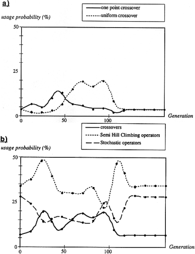
SAGA was run on all the test cases, and the schedules for all the operators were plotted. Figure 6 a and b present some of these results. Figure 6 a shows that the probabilities of being used of the two types of crossover (one point and uniform) evolve according to different schedules. In the early stages, the young population is very heterogeneous and lacks consistency. Thus the uniform crossover can hardly be used. Later in the run, when some order has been created, the uniform crossover can be applied more easily. It then gradually replaces the one point crossover. This graph clearly shows that the two types of crossover are competing with each other, although no extra information regarding the type of the operator is given to the algorithm. All the operators were analysed in the same way, in order to verify that they were needed (data not shown).
Figure
Some operators are stochastic and some work in a semi-hill climbing
way. We verified that these semi-hill climbing operators were not over-weighted
with respect to the other operators. The results are shown in Figure 6
b. This figure clearly reveals that the semi-hill climbing and stochastic
operators behave in a complementary way during the run. During the early
stages, semi-hill climbing operators that easily generate improvements
are favoured. Once all the possible easy improvements have been made, however,
stochastic operators gradually replace the semi-hill climbing ones, opening
the way for new configurations. This alternate use of both types of mutation
is repeated through a series of cycles, until the evolution stops. When
this point is reached, operators find it difficult or impossible to generate
new improvements and they stabilise at their original, default level of
1/22 (when no improvement has been made for some specified number of generations).
Although these schedules vary from one test case to another, the main patterns,
described above, occur consistently. Closely related operators compete
with each other and may display cycles of oscillation. Each possible modification
may be viewed as a niche for which the various operators compete during
the run. It must be emphasised here that these schedules are natural in
the sense that no coding is responsible for the observed phenomenon of
oscillation that we described. These results suggest that SAGA through
the dynamic operator setting is able to optimise the use of each operator
according to its real behaviour.
SAGA and MSA were compared with regard to their ability to optimise OF1. This is the OF that MSA attempts to optimise. For nine of the test cases, we compared the alignments produced by MSA and those generated by SAGA. SAGA was run with default parameter settings. The results shown in Table 1 are the best from three trials. On a larger number of runs it was verified that SAGA reaches this solution in at least one third of the runs. In all the cases, SAGA was able to produce a score at least as good as that produced by MSA (note that the lowest scores are the better ones). In four cases, this score was better. We tried to derive a correlation between the mathematical optimisation of OF1 and its biological relevance. To do so, these four alignments were compared with the structural reference alignments for consistency. This analysis reveals that an improvement of the optimisation consistently correlates with an improvement of the accuracy: the alignments for which SAGA outperforms MSA are more similar to their structural references. Recently, MSA has been upgraded by a newer, faster version but the results are identical ( 7 ).
In principle, MSA can be used to find the guaranteed optimal alignment
for a set of sequences. In practice, however, the parameter settings required
to do so will often be prohibitively expensive in terms of time and memory.
By default, MSA uses heuristic bounds which do not guarantee optimality.
In cases where SAGA achieves a better score than MSA, one can calculate
new bounds from the SAGA alignment and use these to run MSA. In this case,
MSA achieves the same score as SAGA (data not shown). In practice, if you
do not have a higher scoring reference alignment (e.g. from SAGA), adjusting
the bounds is not trivial. If they are set incorrectly, you either do not
get the optimal alignment or MSA runs out of memory. Attempts at finding
better solutions than those found by SAGA by increasing the bounds used
by MSA, failed to find better scoring solutions. Starting with the bounds
calculated from the SAGA alignment, the bounds were increased as much as
possible up to the point where the problem became uncomputable with available
computer time and memory. This suggests that the solutions presented in
Table 1 could
indeed be optimal.
MSA uses quasi-natural gap penalties because of the computational cost of using natural ones. It can be argued that natural gap penalties are more biologically realistic ( 18 ) and we therefore use them for the remaining four test cases. MSA is also severely limited regarding the number and the length of the sequences it can align. In these four test cases, there were too many sequences for MSA to perform its task. Without the MSA reference, it becomes difficult to assess the efficiency of the optimisation. Therefore, we replaced the MSA reference with an alignment produced by CLUSTAL W. It must be stressed here that CLUSTAL W does not explicitly try to optimise any OF. Despite these limitations, by choosing an appropriate set of parameters, we used CLUSTAL W in conditions where it would produce a result as close as possible to the optimisation of OF2. These alignments were compared with those obtained from SAGA while optimising OF2.
Both sets of alignments were then compared to the structural reference alignments of Pascarella ( 29 ). These results are presented in Table 2 and show that in all four test cases SAGA builds an alignment with a better score than CLUSTAL W, regarding OF2. This Table also shows that in three out of four test cases, the alignment generated by CLUSTAL W is less similar to the structural alignment than is that produced by SAGA. These results suggest that with similar types of weights, similar types of substitution cost (Pam 250) and similar range of gap penalties, SAGA performs more accurately than CLUSTAL W on data sets of realistic size.
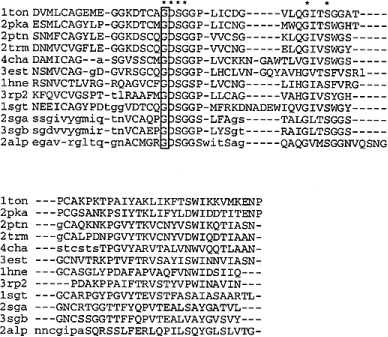
Figure 7 presents the N-terminus portion of the S protease2 test case obtained with SAGA. The reference structural alignment contains 12 completely conserved positions. SAGA is able to reconstitute 11 of these positions while CLUSTAL W only finds 10 of them. Overall, the comparison of the SAGA alignment with the structural reference shows that the main features are accurately found by our algorithm.
Figure
We believe SAGA to be a powerful and flexible tool for sequence alignment. This can be seen by the ability of SAGA to achieve what appear to be optimal alignment scores and by the consistency of our alignments with test cases of known tertiary structure. The consistency of the SAGA alignments with structural reference alignments is mainly a measure of the usefulness of the particular OFs we have tested. Nonetheless, even with the very limited range of OFs that we have tried, SAGA performs extremely well. SAGA is still fairly slow for large test cases (e.g. with >20 or so sequences) but we have made little effort at optimising the program for sheer speed. In the future, it may be desirable to use a hybrid progressive/genetic algorithm approach in order to combine the speed of the former with the accuracy of the latter.
Currently, we seed the starting population of alignments completely randomly. We could use heuristic alignments generated by CLUSTAL W, for example, perhaps with different parameter settings and refine these. We prefer not to, however, as the starting alignments could be trapped in local minima. If the starting alignment is close to the optimal solution, SAGA could be used very easily as an alignment improver. This would provide an easy method for generating hybrid alignments for very large test cases but we have not evaluated SAGA in detail in this respect.
Genetic algorithms have been used successfully as a practical way to solve many computationally difficult problems. They are intellectually satisfying in their simplicity and the way they attempt to mimic biological evolution. From the point of view of multiple sequence alignment, the use of stochastic optimisation methods has proved to be difficult with just a few exceptions ( 9 , 32 ). We found that a simple GA, applied in a straightforward fashion to the alignment problem was not very successful. The main device which allowed us to efficiently reach very high quality solutions was to use a large number of mutational and crossover operators and to automatically schedule them. At first glance, this is not very satisfactory in that it makes the method seem very complicated and cumbersome. Multiple alignment, however, is not a simple problem. The most useful of our operators are the ones which appear most based in biological reality e.g. moving blocks using the tree as a guide. In reality, during the course of the evolution of a sequence family, many different evolutionary events may take place. The automatic scheduling has a further advantage. Should it turn out, in the future, that SAGA is not very efficient at handling certain types of situation, it is a simple matter to invent some new operators designed specifically for the problem and to slot them into the existing scheme. The automatically assigned probabilities of usage at different stages in the alignment give a direct measure of usefulness or redundancy for a new operator.
The second major reason for using GAs in the context of multiple alignment is the complete freedom to use any OF one can think of. This is perhaps the most important single feature of the approach. One key to successfully tackling the multiple alignment problem is to have a good measure of multiple alignment quality. The GA used in SAGA offers the opportunity to implement and test new OFs.
After sequence alignment, there are two related questions which one
might wish to ask. First one might like to know if the alignment is significant
with respect to some statistical model e.g. one might like to know the
probability of observing any particular alignment by chance alone. This
is a very difficult problem which has solutions for two sequences under
certain conditions ( 30
). The second question is how stable is the alignment or which pieces
of the alignment are stable i.e. are there alternative alignments with
similar alignment scores? This is important if one is to usefully interpret
new alignments and there are some solutions, again, for just two sequences
( 33 ). A by
product of the GA strategy in SAGA is a measure of consistency for each
column in the final alignment. This shows which columns are stable and
which ones have high scoring alternative arrangements. The consistency
is derived by counting how often a particular column occurs in the 100
alignments of a SAGA population during or after optimisation. We have no
statistical interpretation of this consistency measure but it is an extremely
useful by product of the SAGA alignment process at no extra computational
cost.
We wish to thank Stephen Altschul for advice on using MSA.